
Energy Distance: Cross and Within Distribution Terms
2026-11-18
Energy Distance: Cross and Within Distribution Terms
Energy distance compares distributions by combining average cross-distribution separation with average separation inside each distribution. The subtraction of the two within-distribution terms is essential: the quantity is not simply the average distance between every observation in one group and every observation in another. Its name describes a statistical construction and does not mean electrical consumption or mechanical work.
Three expectations appear before the square root
The SciPy 1.16 energy_distance documentation defines the one-dimensional distance as the square root of twice the expected absolute difference between X and Y, minus the expected absolute difference between independent X and X-prime draws, minus the corresponding expectation for Y and Y-prime.
X and X-prime follow the first distribution; Y and Y-prime follow the second. For an empirical distribution with equally weighted listed values, independent draws include the possibility of selecting the same listed value twice. The zero diagonal terms therefore belong in the within-distribution expectation. Replacing that expectation with an average over only distinct index pairs would calculate a different expression.
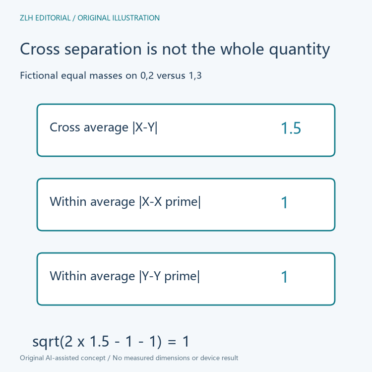
Compute an invented two-point comparison explicitly
Let the first fictional distribution put equal mass on zero and two, and the second put equal mass on one and three. The four cross absolute differences are one, three, one and one, so their average is one and a half. Within the first distribution, the four ordered differences are zero, two, two and zero, averaging one. The second distribution also has a within average of one.
The squared quantity is consequently twice one and a half minus one minus one, which is one. Its square root is one. The example lists all pairs so that the factor of two and the two subtractions remain visible. Neither the input values nor the resulting distance come from a robot-learning experiment.
Identical distributions cancel without requiring zero spread
If both inputs instead represent the same equally weighted distribution on zero and two, the cross expectation equals each within expectation. The same expression becomes twice one minus one minus one, giving zero. Individual draws can differ by two even though the two distributions being compared agree.
This is why spread alone should not be mistaken for separation between distributions. A broad empirical distribution compared with itself has zero distance. Conversely, a comparison needs the probability masses as well as the locations: using the same support values with different weights can describe different distributions.
Normalized weights describe mass rather than a raw total
The interface allows one weight per listed value. The sum must be positive and finite so that the weights can be normalized. Scaling every weight within one distribution by the same positive factor leaves its normalized masses unchanged. It should therefore leave the represented distribution unchanged, rather than multiplying the distance as though the weights were an unnormalized count total.
Likewise, listing each value twice with equal weights represents the same empirical mass allocation as the original equally weighted list. This observation is about a distributional calculation, not a claim that duplicating observations creates more independent evidence for a statistical test. The interface returns a distance rather than a significance probability.
The cited implementation uses cumulative distributions
The original SciPy implementation computes this one-dimensional quantity through the integral of the squared difference between cumulative distribution functions. It sorts the support locations, obtains the interval widths and evaluates cumulative masses over those intervals. The energy-distance wrapper multiplies that integral's square root by the square root of two.
This route agrees with the expectation definition without constructing every pairwise difference matrix. The pair table in the illustration is a way to understand a tiny example, not a claim that the library allocates that table internally. It is also important to retain the outer square root: some literature uses the squared quantity under a related name, so values from differing conventions require careful comparison.
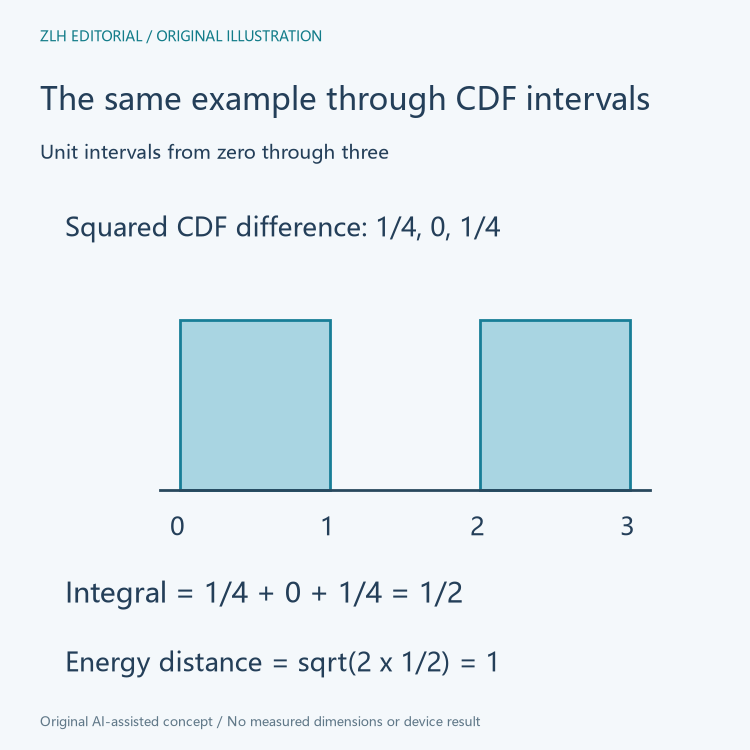
For the fictional two-point comparison, the cumulative distributions differ by one half between zero and one, agree between one and two, and differ by one half again between two and three. Squaring and integrating gives one quarter plus zero plus one quarter, or one half. Multiplying that integral by two and taking the square root again gives one. This second calculation checks the same distributional example through intervals rather than through observation pairs.
A data note should state the support values, weighting convention and square-root convention before interpreting a number. The examples here establish arithmetic only and do not select a model, diagnose a device or measure training quality. Related explanations appear in the learning-data methods section and the technical article archive.