Spectral Leakage: Why One Tone Spreads Across Bins

Spectral Leakage can make a single tone appear in several positions of a discrete spectrum. A finite recording supplies only a segment of the original signal. If that segment contains a noninteger number of cycles of a tone, the tone may fall between the discrete frequencies evaluated by the transform. The resulting spread can belong entirely to the observation and analysis, even when the example signal has one constant frequency.

A finite record produces a shaped spectrum

The SciPy signal processing tutorial starts with a sine restricted to a finite time interval. Mathematically, retaining the signal inside that interval and setting it to zero outside is multiplication by a rectangular window. The continuous Fourier transform of that observation has a peak region and smaller lobes around each of the sine's positive and negative frequency components. The lobes arise because the signal has been confined to a finite interval.

Sampling the record and taking a discrete Fourier transform evaluates a spectrum at specific frequencies. At any one evaluated frequency, the transform combines the samples after applying a matching sequence of phase shifts. If those shifts exactly match the advance of an ideal complex tone, all contributions line up. For a tone between two evaluated frequencies, the contribution phases usually do not cancel completely at neighboring bins.

A matching bin and a half-bin offset look different

Consider an invented record with 32 equally spaced samples of a single complex tone. If it completes exactly six cycles over the 32 sample intervals defining the transform period, the rectangular-window result concentrates in bin six. At each other bin, the equally spaced phase contributions cancel. If the tone instead completes six and a half cycles over that same period, the bin frequencies stay fixed and the tone lies halfway between bins six and seven.

The first illustration shows the resulting magnitudes. In the second case, several bins have visible values even though the time-domain example still has only one complex tone. This is a statement about the finite record and the transform basis. A real sinusoid would have positive and negative frequency components, so the complex example isolates the behavior of one component for the drawing.

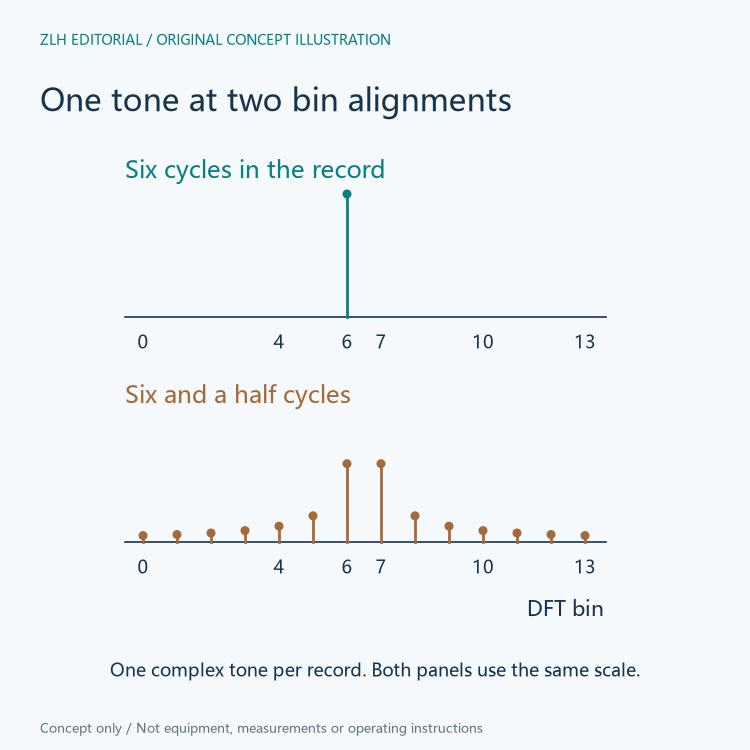
The rectangular-window transform of six exact cycles has one visible bin, while a six-and-a-half-cycle tone spreads across bins. — Original transform of two synthetic complex tones. Source: Zhilianhai editorial desk, original AI-assisted conceptual illustration; no real product or measured data.

The transform period in this example is the time from the first sample to the next repetition of that first sample. It spans 32 sample intervals. The final measured sample arrives one interval before that repetition. Requiring the final stored sample to equal the first would impose a different condition.

A taper changes the shape of the spread

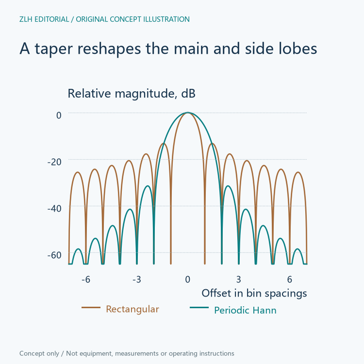
A tapered window multiplies the retained samples by different weights before the transform. The Hann window described in SciPy is a raised-cosine taper. Its weights are smaller near the edges and larger toward the middle. The tutorial explains that tapering commonly lowers distant side lobes while making the central lobe wider. In this setting, side lobes are smaller peaks away from the tone, while the main lobe is the central response around it.

The second figure compares responses of a rectangular window and a periodic Hann window at the same record length. Each is normalized to its own zero-offset response. For the Hann example, the response extends farther before its first null, while the side lobes farther away are lower. A weaker nearby component can be obscured by the wider main lobe, while a weaker component farther away can become easier to distinguish against lower side lobes.

Two 32-sample window responses, each scaled to its zero-offset magnitude, show a wider main lobe and lower distant side lobes for the Hann taper. — Original window response curves, clipped at the figure floor. Source: Zhilianhai editorial desk, original AI-assisted conceptual illustration; no real product or measured data.

Window weighting also changes the amplitude scale

The tutorial divides windowed transform magnitudes by the absolute sum of the window weights when forming its amplitude spectrum. The reason can be seen from a matching complex tone. At the matching bin the phase terms cancel each other's rotation, leaving the tone's amplitude multiplied by the sum of the weights. A window with lower average weight therefore changes the raw magnitude even when the tone and record length are identical.

That scale adjustment does not move the tone onto a bin. It gives a defined magnitude reference for comparisons at a matching frequency. If the tone is between bins, the nearest values still sample the lobe at nonzero offsets. For this reason, a comparison of peak heights needs to retain both the weighting and the amplitude convention.

Keep the record and the analysis choices together

For an interpretable plot, identify the measured interval, the window used, and the magnitude convention. If two curves are being compared, make clear whether they come from the same samples. A change in the spread around a peak can reflect a change in the window or the alignment of the tone with evaluated frequencies, even before considering any change in the original source.